Without Using Seurat Object
Introduction
This tutorial demonstrates how to use the SpaCCI package for analyzing spatial cell-cell interactions using an example of spot-level datasets.
Part I: Data Input, Processing and Initialization.
We first load the SpaCCI package:
library(SpaCCI)
Please still load the Tutorial_example_data.rda for getting the interest_region_Spot_IDs for regional analysis section.
load(system.file("extdata", "Tutorial_example_data.rda", package = "SpaCCI"))
Prepare required input data for SpaCCI analysis
Below, we demonstrate how to prepare these datasets using the example data provided in the Data Section.
(A) Normalized gene expression data frame
# Read normalized spot-level gene expression data.
normalized_gene_spot_df <- read.csv("~/normalized_gene_spot_df.csv")
# Make the gene names be the row names
rownames(normalized_gene_spot_df) <- normalized_gene_spot_df$X
# Make the column name contains only spot IDs
normalized_gene_spot_df <- normalized_gene_spot_df[,-1]
(B) Prepare the cell type proportion data frame.
# Read spot-level cell type proportion data.
cell_prop_df <- read.csv("~/cell_prop_df.csv")
# Make the spot IDs be the row names
rownames(cell_prop_df) <- cell_prop_df$X
# Make the column names contains only cell type names
cell_prop_df <- cell_prop_df[,-1]
(C) Prepare the spatial coordinates data frame.
# Read spot-level spatial coordinates data.
cell_prop_df <- read.csv("~/spatial_coords_df.csv")
# Make the spot IDs be the row names
rownames(spatial_coords_df) <- spatial_coords_df$X

# Make the column names contains `c("imagerow","imagecol")`
# If your spatial coordinates are `c("x","y")`,
# then PLEASE rename to `c("imagecol","imagerow")`
# If your spatial coordinates are `c("y","x")`,
# then PLEASE rename to `c("imagerow","imagecol")`

spatial_coords_df <- spatial_coords_df[,-1]
(D) Ensure consistency between all the three data frames.
# Check that the spot IDs in `cell_prop_df` and `spatial_coords_df` match the column names in `normalized_gene_spot_df`.
stopifnot(setdiff(rownames(cell_prop_df), colnames(normalized_gene_spot_df)) == character(0))
stopifnot(setdiff(rownames(spatial_coords_df), colnames(normalized_gene_spot_df)) == character(0))
stopifnot(setdiff(rownames(spatial_coords_df), rownames(cell_prop_df)) == character(0))

# The above checks confirm that the spot IDs are consistent across the gene expression and cell type proportion data frames,
# ensuring they are ready for SpaCCI analysis.

# If not then we make them the same
colnames(normalized_gene_spot_df) <- rownames(cell_prop_df)
Now we have prepared the data for SpaCCI analysis.
Part II: Access the Ligand-Receptor Interaction Database
We identify possible Ligand-Receptor interactions that might happen on the tissue slides according to the gene expression data.
# Identify Possible Ligand-Receptor Pairs for Cell-Cell Communication
# Specifying the species ("Human" or "Mouse").
# Database options include "CellChat", "CellPhoneDB", "Cellinker", "ICELLNET", and "ConnectomeDB".
# We use the cellchat database, for more information, run '? LR_database' .
LRDB <- LR_database("Human", "CellChat", normalized_gene_spot_df)
Part III: Inferring Cell-Cell Interaction Analysis
(A) Global analysis
Here we first run the global analysis on the whole slide, and plot the overall results using heatmap.
####### global analysis. ###########
# ?run_SpaCCI
result_global <- run_SpaCCI(gene_spot_expression_dataframe = normalized_gene_spot_df,
                             spot_cell_proportion_dataframe = cell_prop_df,
                             spatial_coordinates_dataframe = spatial_coords_df,
                             LR_database_list = LRDB,
                             analysis_scale = "global")

## [1] "writing data frame"

# ?plot_SpaCCI_heatmap
# plot the result heatmap, we set the significant cutoff alpha = 0.05,
# If you want the details on the heatmap, please specify return_tables = TRUE.
p <- plot_SpaCCI_heatmap(SpaCCI_Result_List = result_global,
                    symmetrical = FALSE, cluster_cols = FALSE, return_tables = FALSE,
                    cluster_rows = FALSE, cellheight = 15, cellwidth = 15,
                    specific_celltypes = c(colnames(cell_prop_df)), alpha = 0.05,
                    main= "Significant Cell-Cell Interaction Count")
print(p)

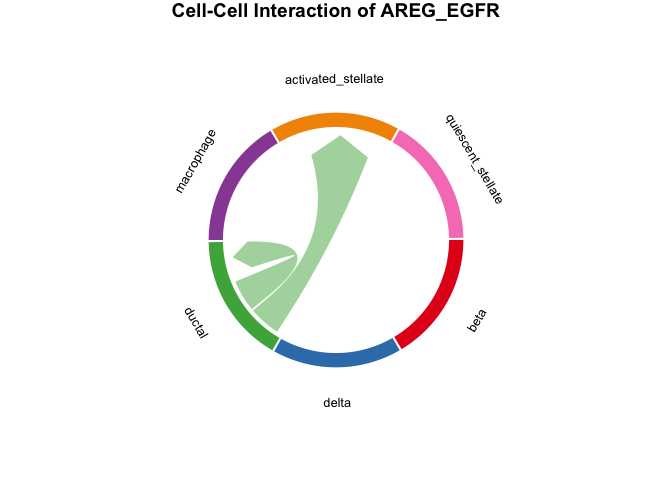
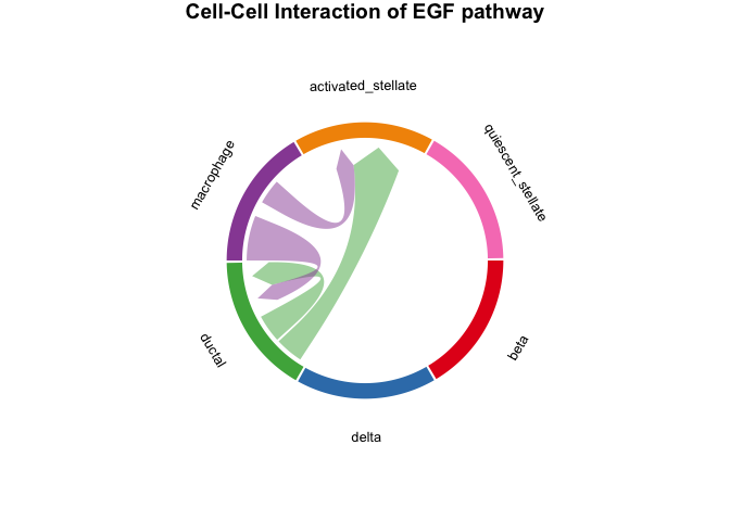
Then we could plot the chord Diagram by specifying specific Ligand-Receptor pair or Pathway name.
- NOTE: When specifying specific Ligand-Receptor pair or Pathway
name please check the
result_global$pvalue_dffor the details on Ligand-Receptor pair and Pathway name.
# plot the result with chordDiagram while selecting specific Ligand-Receptor pair name
plot_SpaCCI_chordDiagram(SpaCCI_Result_List = result_global,
                         specific_celltypes = c(colnames(cell_prop_df)),
                         L_R_pair_name  = "AREG_EGFR")
# plot the result with chordDiagram while selecting specific pathway name
plot_SpaCCI_chordDiagram(SpaCCI_Result_List = result_global,
                  specific_celltypes = c(colnames(cell_prop_df)),
                  pathway_name  = "EGF")
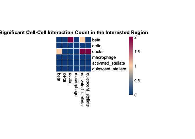
(B) Regional analysis
Here we run the regional analysis on the whole slide with selected
interest_region_Spot_IDs, and plot the overall results using heatmap.
# regional analysis
result_regional <- run_SpaCCI(gene_spot_expression_dataframe = normalized_gene_spot_df,
                            spot_cell_proportion_dataframe = cell_prop_df,
                            spatial_coordinates_dataframe = spatial_coords_df,
                            LR_database_list = LRDB,
                            analysis_scale = "regional",
                            region_spot_IDs = interest_region_Spot_IDs)

## [1] "writing data frame"

# plot the result heatmap
plot_SpaCCI_heatmap(SpaCCI_Result_List = result_regional,
                    symmetrical = FALSE, cluster_cols = FALSE, return_tables = FALSE,
                    cluster_rows = FALSE, cellheight = 15, cellwidth = 15,
                    specific_celltypes = c(colnames(cell_prop_df)), alpha = 0.05,
                    main= "Significant Cell-Cell Interaction Count in the Interested Region")
(C) Local analysis
Finally we run the local analysis on the whole slide with specifying
specific_LR_pair.
NOTE: Local analysis aim to find the localized interaction hotspots, if you find the result are unable to show the hotspots, you could adjust the neighborhood_radius to make it larger.
# local analysis
result_local <- run_SpaCCI(gene_spot_expression_dataframe = normalized_gene_spot_df,
                           spot_cell_proportion_dataframe = cell_prop_df,
                           spatial_coordinates_dataframe = spatial_coords_df,
                           LR_database_list = LRDB,
                           specific_LR_pair = "EDN2_EDNRA",
                           analysis_scale = "local",
                           local_scale_proportion = 1,
                           neighborhood_radius = 2.5)

## [1] "Now analyzing localized detection using 100% of spots in the whole slide, with a radius of 2.5."
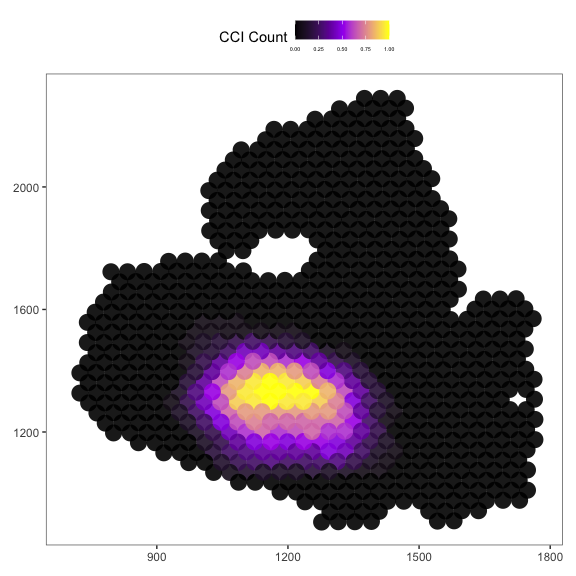
Then we plot the localized plot to access the local signalling hotspot.
# Please use the spatial_coords_df
plot_SpaCCI_local(spatial_coordinates_dataframe = spatial_coords_df,
                  SpaCCI_local_Result_List = result_local,
                  Ligand_cell_type = "ductal",
                  Receptor_cell_type = "activated_stellate",
                  spot_plot_size = 6)

## [1] "plotting using image spatial coordinates"