Using Seurat Object
Introduction
This tutorial demonstrates how to use the SpaCCI package for analyzing spatial cell-cell interactions using an example Seurat 10X Visium dataset.
Part I: Data Input, Processing and Initialization.
Here we demonstrate using our example - 10X Visium dataset - with an Seurat object and the cell type proportion data.
library(SpaCCI)
# Load the example data
load(system.file("extdata", "Tutorial_example_data.rda", package = "SpaCCI"))
Prepare required input data for SpaCCI analysis
SpaCCI requires two main input datasets:
- Gene Expression Data: A spot-level data frame with genes as row names and spot IDs as column names.
- Cell Type Proportion Data: A spot-level data frame with spot IDs as row names and cell type labels as column names.
Below, we demonstrate how to prepare these datasets using the example
data provided in the Tutorial_example_data.rda file.
# After loading Tutorial_example_data.rda, the following objects should be available:
# - Example_Seurat: A Seurat object containing 10X Visium data with an associated image.
# - cell_prop_df: A data frame containing spot-level cell type proportions.
# - interest_region_Spot_IDs: Spot IDs for conducting "regional" analysis.
(A) Normalize the Seurat data and extract the gene expression data frame
# Normalize the Seurat object.
Example_Seurat <- NormalizeData(Example_Seurat)

# Extract the gene expression data frame.
gene_spot_df <- as.data.frame(Example_Seurat@assays$Spatial@data)

# Inspect the first few rows and columns of the gene expression data frame.
head(gene_spot_df[c(1:3), c(1:3)])

##       AAACGAGACGGTTGAT-1 AAACTGCTGGCTCCAA-1 AAAGGGATGTAGCAAG-1
## CSF1R            0.00000                  0           6.813544
## EDNRB            6.34214                  0           6.813544
## EDNRA            6.14186                  0           0.000000

# The gene expression data frame for SpaCCI should have the following structure:
#
#               spot_id_1   spot_id_2   spot_id_3  ......
# Gene_name1
# Gene_name2
# Gene_name3
#   .....

# Alternatively, you can use SCTransform to normalize the data:
# Example_Seurat <- SCTransform(Example_Seurat, assay = "Spatial", verbose = FALSE)
# gene_spot_df <- as.data.frame(Example_Seurat[["SCT"]]@data)
(B) Prepare the cell type proportion data frame.
# The row names of `cell_prop_df` should be set to the spot IDs.
rownames(cell_prop_df) <- cell_prop_df$X
cell_prop_df <- cell_prop_df[, -1]

# Inspect the first few rows of the cell type proportion data frame.
head(cell_prop_df[c(1:3), ])

##                         beta      delta    ductal macrophage activated_stellate
## AAACGAGACGGTTGAT-1 0.2500000 0.08333333 0.4166667 0.00000000         0.08333333
## AAACTGCTGGCTCCAA-1 0.5833333 0.16666667 0.2500000 0.00000000         0.00000000
## AAAGGGATGTAGCAAG-1 0.2500000 0.00000000 0.5833333 0.08333333         0.00000000
##                    quiescent_stellate
## AAACGAGACGGTTGAT-1         0.16666667
## AAACTGCTGGCTCCAA-1         0.00000000
## AAAGGGATGTAGCAAG-1         0.08333333

# The cell type proportion data frame for SpaCCI should have the following structure:
#
#               celltype1   celltype2   celltype3  ......
# spot_id_1
# spot_id_2
# spot_id_3
#   .....
(C) Ensure consistency between the Seurat object and the data frames.
# Check that the spot IDs in `cell_prop_df` match the column names in `gene_spot_df` and `Example_Seurat`.
stopifnot(setdiff(rownames(cell_prop_df), colnames(gene_spot_df)) == character(0))
stopifnot(setdiff(rownames(cell_prop_df), colnames(Example_Seurat)) == character(0))

# The above checks confirm that the spot IDs are consistent across the gene expression and cell type proportion data frames,
# ensuring they are ready for SpaCCI analysis.
Prepare the spatial coordinates.
# If using a Seurat Object loaded with Load10X_Spatial
# For example:
# Seurat_Object <- Load10X_Spatial(
#   data.dir = "/path/to/data/",
#   filename = "your_data_file.h5",
#   assay = "Spatial",
#   slice = "slice1",
#   filter.matrix = TRUE,
#   to.upper = FALSE,
#   image = NULL
# )
#
# You can directly use the `GetTissueCoordinates` function as follows:
# spatial_coords_df <- GetTissueCoordinates(Seurat_Object, image = "slice1")
#
# However, if you have an existing Seurat object (e.g., Example_Seurat) with the "slice1" image loaded:

# Extract the tissue coordinates from the Seurat object
spatial_coords_df <- as.data.frame(Example_Seurat@images$slice1$centroids)

# Check the first few rows of the spatial coordinates data frame
head(spatial_coords_df) # It should have columns named "x" and "y"

##      x    y
## 1 1196 1432
## 2 1419 1763
## 3 1521 1074
## 4  909 1724
## 5  872 1658
## 6 1380 1828

# Rename columns "x" to "imagecol" and "y" to "imagerow"
colnames(spatial_coords_df) <- c("imagecol", "imagerow")

# Add a "Spot_ID" column that matches the column names in `Example_Seurat` and `gene_spot_df`,
# and the row names in `cell_prop_df`
spatial_coords_df$Spot_ID <- colnames(Example_Seurat)

# Set the row names of the `spatial_coords_df` to be the `Spot_ID`
rownames(spatial_coords_df) <- spatial_coords_df$Spot_ID

# Check the final structure of the `spatial_coords_df` to ensure it has
# columns "imagecol", "imagerow", and "Spot_ID", with "Spot_ID" as row names
head(spatial_coords_df)

##                    imagecol imagerow            Spot_ID
## AAACGAGACGGTTGAT-1     1196     1432 AAACGAGACGGTTGAT-1
## AAACTGCTGGCTCCAA-1     1419     1763 AAACTGCTGGCTCCAA-1
## AAAGGGATGTAGCAAG-1     1521     1074 AAAGGGATGTAGCAAG-1
## AAAGTGTGATTTATCT-1      909     1724 AAAGTGTGATTTATCT-1
## AAAGTTGACTCCCGTA-1      872     1658 AAAGTTGACTCCCGTA-1
## AAATACCTATAAGCAT-1     1380     1828 AAATACCTATAAGCAT-1
Part II: Access the Ligand-Receptor Interaction Database
We identify possible Ligand-Receptor interactions that might happen on the tissue slides according to the gene expression data.
# Identify Possible Ligand-Receptor Pairs for Cell-Cell Communication
# Specifying the species ("Human" or "Mouse").
# Database options include "CellChat", "CellPhoneDB", "Cellinker", "ICELLNET", and "ConnectomeDB".
# We use the cellchat database, for more information, run '? LR_database' .
LRDB <- LR_database("Human", "CellChat", gene_spot_df)
Part III: Inferring Cell-Cell Interaction Analysis
(A) Global analysis
Here we first run the global analysis on the whole slide, and plot the overall results using heatmap.
####### global analysis. ###########
# ?run_SpaCCI
result_global <- run_SpaCCI(gene_spot_expression_dataframe = gene_spot_df,
                             spot_cell_proportion_dataframe = cell_prop_df,
                             spatial_coordinates_dataframe = spatial_coords_df,
                             LR_database_list = LRDB,
                             analysis_scale = "global")

## [1] "writing data frame"

# ?plot_SpaCCI_heatmap
# plot the result heatmap, we set the significant cutoff alpha = 0.05,
# If you want the details on the heatmap, please specify return_tables = TRUE.
p <- plot_SpaCCI_heatmap(SpaCCI_Result_List = result_global,
                    symmetrical = FALSE, cluster_cols = FALSE, return_tables = FALSE,
                    cluster_rows = FALSE, cellheight = 15, cellwidth = 15,
                    specific_celltypes = c(colnames(cell_prop_df)), alpha = 0.05,
                    main= "Significant Cell-Cell Interaction Count")
print(p)

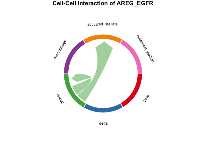
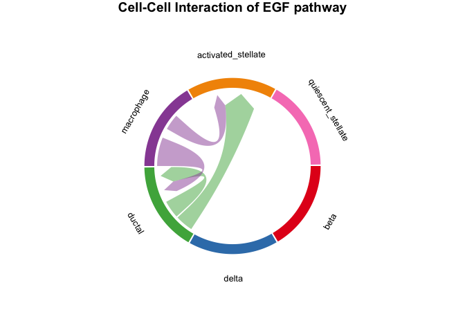
Then we could plot the chord Diagram by specifying specific Ligand-Receptor pair or Pathway name.
- NOTE: When specifying specific Ligand-Receptor pair or Pathway
name please check the
result_global$pvalue_dffor the details on Ligand-Receptor pair and Pathway name.
# plot the result with chordDiagram while selecting specific Ligand-Receptor pair name
plot_SpaCCI_chordDiagram(SpaCCI_Result_List = result_global,
                         specific_celltypes = c(colnames(cell_prop_df)),
                         L_R_pair_name  = "AREG_EGFR")
# plot the result with chordDiagram while selecting specific pathway name
plot_SpaCCI_chordDiagram(SpaCCI_Result_List = result_global,
                  specific_celltypes = c(colnames(cell_prop_df)),
                  pathway_name  = "EGF")
(B) Regional analysis
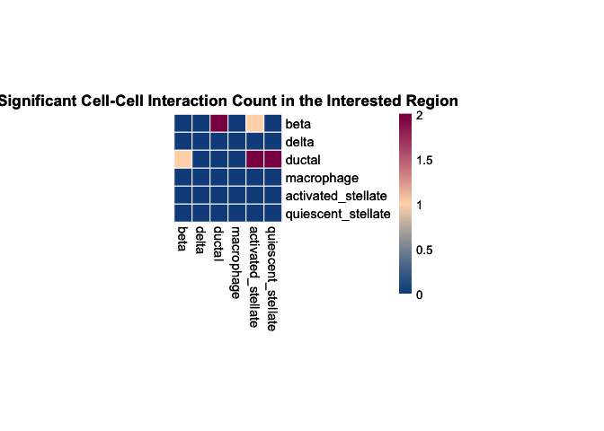
Here we run the regional analysis on the whole slide with selected
interest_region_Spot_IDs, and plot the overall results using heatmap.
# regional analysis
result_regional <- run_SpaCCI(gene_spot_expression_dataframe = gene_spot_df,
                            spot_cell_proportion_dataframe = cell_prop_df,
                            spatial_coordinates_dataframe = spatial_coords_df,
                            LR_database_list = LRDB,
                            analysis_scale = "regional",
                            region_spot_IDs = interest_region_Spot_IDs)

## [1] "writing data frame"

# plot the result heatmap
plot_SpaCCI_heatmap(SpaCCI_Result_List = result_regional,
                    symmetrical = FALSE, cluster_cols = FALSE, return_tables = FALSE,
                    cluster_rows = FALSE, cellheight = 15, cellwidth = 15,
                    specific_celltypes = c(colnames(cell_prop_df)), alpha = 0.05,
                    main= "Significant Cell-Cell Interaction Count in the Interested Region")
(C) Local analysis
Finally we run the local analysis on the whole slide with specifying
specific_LR_pair.
NOTE: Local analysis aim to find the localized interaction hotspots, if you find the result are unable to show the hotspots, you could adjust the neighborhood_radius to make it larger.
# local analysis
result_local <- run_SpaCCI(gene_spot_expression_dataframe = gene_spot_df,
                           spot_cell_proportion_dataframe = cell_prop_df,
                           spatial_coordinates_dataframe = spatial_coords_df,
                           LR_database_list = LRDB,
                           specific_LR_pair = "EDN2_EDNRA",
                           analysis_scale = "local",
                           local_scale_proportion = 1,
                           neighborhood_radius = 2.5)

## [1] "Now analyzing localized detection using 100% of spots in the whole slide, with a radius of 2.5."
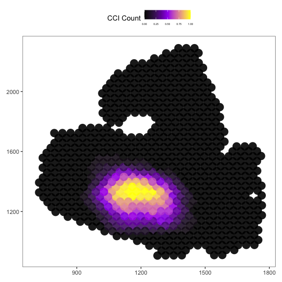
Then we plot the localized plot to access the local signalling hotspot.
# if you have the Seurat Object with image
plot_SpaCCI_local(Seurat_Object = Example_Seurat,
                  SpaCCI_local_Result_List = result_local,
                  Ligand_cell_type = "ductal",
                  Receptor_cell_type = "activated_stellate",
                  spot_plot_size = 6)

## [1] "plotting using Seurat image"

## Scale for fill is already present.
## Adding another scale for fill, which will replace the existing scale.
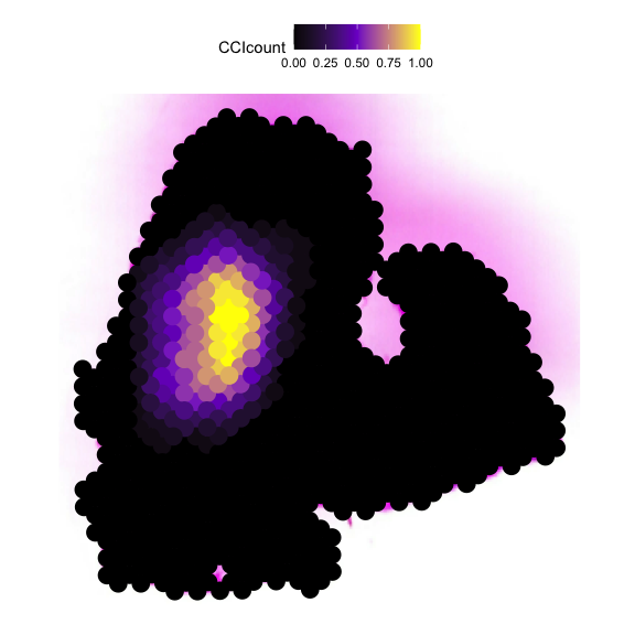
# if you DON'T have the Seurat Object with image, Please use the spatial_coords_df
plot_SpaCCI_local(spatial_coordinates_dataframe = spatial_coords_df,
                  SpaCCI_local_Result_List = result_local,
                  Ligand_cell_type = "ductal",
                  Receptor_cell_type = "activated_stellate",
                  spot_plot_size = 6)

## [1] "plotting using image spatial coordinates"
